Imposing boundary conditions via Nitsche’s Method
Imposing boundary conditions via Nitsche’s Method
Several problems analyzed in engineering can be mathematically described by differential equations that become complex when trying to portray with fidelity the analyzed phenomenon, as well as the complexity of the geometry. Numerical methods, together with computation development, are important tools for the approximate solution of these problems. Among these methods, the Finite Element Method (FEM) and the Meshless Method (MM) are the most outstanding.
FEM is an already consolidated method, described by Moreira and Pitangueira (2006) as a method that presupposes the division of the study domain into interconnected sub-domains, called finite elements. Its formulation is usually based on the displacements, when applied in the structural analysis, that is, for each of the nodes that form the elements there is an interpolation function to calculate their respective displacements. It is necessary to establish hypotheses related to the deformations regime (deformations and displacements relations), small or large deformations and the material behavior (stresses and deformations relations). These three hypotheses are considered in obtaining the nodal equilibrium equations of the element. However, this method is, by definition, a mesh dependent method, and when discretizing the domain in elements there are some difficulties in the analysis of problems with discontinuity, large deformations or elevated gradients.
The MM arise as an alternative to these difficulties, since these methods establish a coherent discretization between the formulation of the algebraic equations and the singularity phenomena, partly because they do not use a predefined mesh, but also because they describe nodal displacements in a more complex manner, capable of capturing more abrupt variations in the nodal quantities evaluated. The discretization of the domain is done only by points, as explained by Liu (2009). This guarantees the mesh independence, one of the main characteristics of the MM, which provides greater ease in treating phenomena such as discontinuity and fracture. Among the MM, the main methods are: Element Free Galerkin (EFG), Reproducing Kernel Particle Method (RKPM) Liu et al. (1995), Smoothed Particle Hydrodynamics (SPH) Monaghan (1992) and Meshless Local Petrov-Galerkin (MLPG) Atluri and Zhu (1998). Among these methods, EFG stands out in this work, although it does not depend on mesh to discretize the geometry, it needs integration cells, known as background cells, to perform integration in the domain.
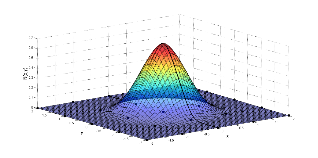
Although they are robust and efficient methods, they present some disadvantages in relation to FEM. According to Silva (2012), because they more complex function-based formulation, compared to FEM that are restricted to polynomial shape functions, a higher order integration is necessary, thus increasing the computational cost. These shape functions, in some MM, do not present the property of the Kronecker Delta, as shown graphically in Figure 1. Thus, the imposition of the Direchlet boundary conditions is not trivial, as in MEF
Figure 1
By demonstrating the difficulty in imposing the essential contour conditions, according to Fernandez-Mendez and Huerta (2003) one can divide the techniques to perform the imposition in two groups. The first one is based on modifications of the weak form, among which the Lagrange Multiplier (ML), the Penalty Method (PM) and the Nitsche’s Method (MN) stand out. The second group is characterized by methods that establish modifications of the shape functions, and brings as an example the coupling with finite elements. The different formulations are shown in Figure 2.
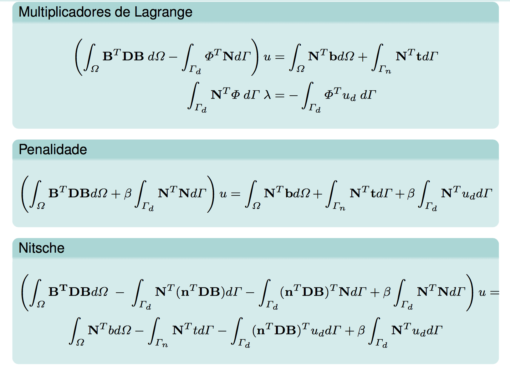
Figure 2 – Equations 1, 2 and 3
The objective of this work with Professor Ramon Silva is to implement, in the INSANE environment, the Nitsche method as a strategy for the imposition of boundary condition for the EFG, implemented by Silva (2012). In addition, the accuracy of the results is compared with that obtained using the strategies already implemented in the software and with the exact solution of one of the problems analyzed, which is available in the literature. Based on the studies in the work of Augarde and Deeks (2008), a beam of rectangular cross section was initially discretized in 85 regularly distributed nodes with 4×16 integration cells (Figure 3).
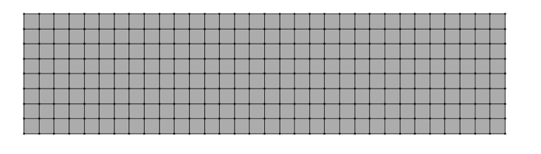
Figure 3
The influence domain of each node is rectangular in size, 5% larger than the distance between the nodes of the geometric discretization. The material used, as well as the geometry of the example, followed what was proposed in the work of Augarde and Deeks (2008), with modulus of elasticity E = 1000 uf/ua, Poisson ν = 0.25 and dimensions of D = 2 uc, L = 8 uc and unit thickness, I = D3/12, so the second-order moment of inertia is 0.667 uc3. A stress with normal parabolic distribution to the Y direction was applied to the right-side edge, according to Equation 4. The analysis model is a plane stress analysis. As boundary condition, on the left-hand side was imposed the analytical displacement of the problem as described in Equations 5 and 6. In these equations X and Y represent the coordinates according to the Cartesian system positioned at the center of the beam height and starting the X axis at the left edge, as shown in Figure 4. In order for these natural and essential boundary conditions to be correctly understood in the INSANE, it was necessary to apply the equivalent load to the stress described in 4 as a nodal load with an equivalent value obtained when integrating the area of influence of each node. The calculated displacement analysis values, but also Equations 5 and 6, were also prescribed as nodal displacements.
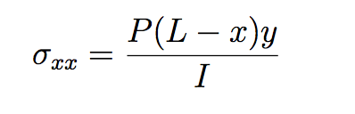
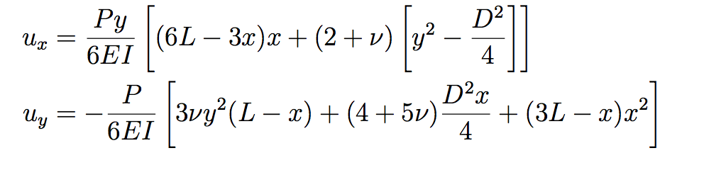 Figure 4 – Equations 4, 5 and 6
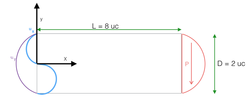
Figure 5
Comparing displacements in the Y direction obtained with the different boundary conditions methods, as: penalty method, Lagrange multipliers and Nietsche’s method, as well as in comparison with FEM results. Then, Graphic 1 shows the comparative values to the analytical result in the different discretizations found in the edge.
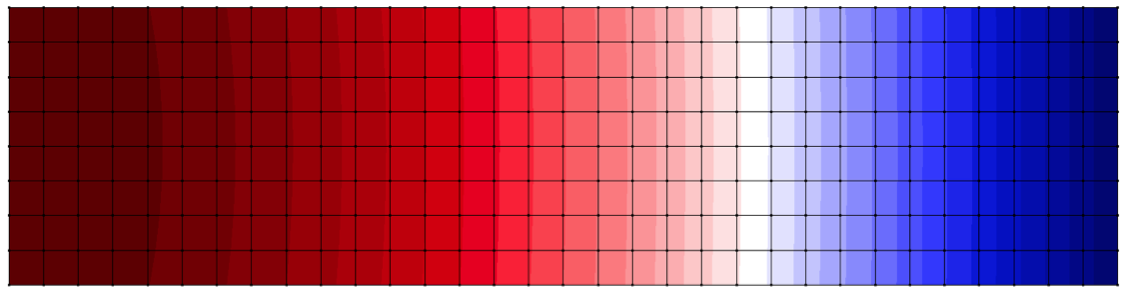
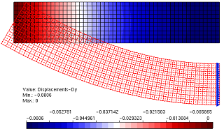
Figure 6 – Displacement in Y direction via FEM
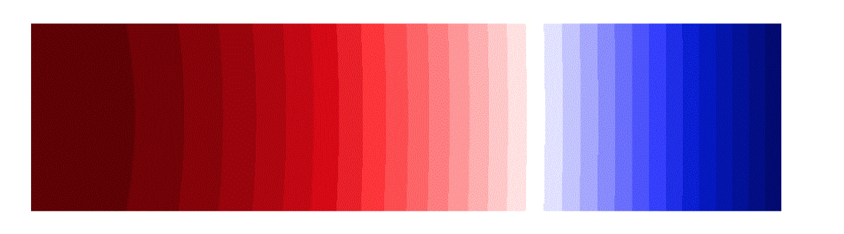
Figure 7 – Displacement in Y direction via Lagrange Multiplier Method
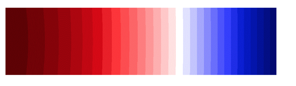
Figure 8 – Displacement in Y direction via Penalty Method β=1000
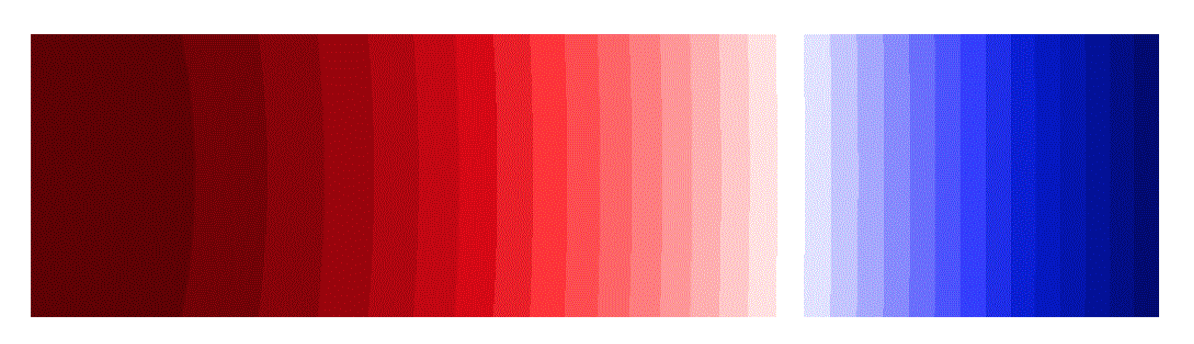
Figure 9 – Displacement in Y direction via Nietsche’s Method β=1000
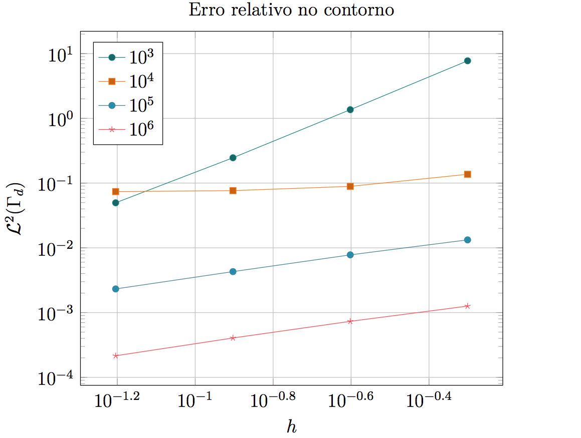
Graphic 1
It can be observed, therefore, that the Nitsche method is able to impose the prescribed boundary conditions in a satisfactory way, being a method that improves its approximation with increases lower than necessary for the application of the boundary condition by the Method of Penalty. Although its accuracy is strongly related to the order of magnitude of the factor β, it can be observed that a lower value was required, to obtain a smaller error in the calculated displacements when compared to the displacements obtained in an analytical way, than what is necessary for Penalty Method satisfies the same accuracy.
References
- Atluri, S. N. and Zhu, T. (1998), ‘A new Meshless Local Petrov-Galerkin (MLPG) approach in computational mechanics’, Computational Mechanics 22(2), 117–127.
- Augarde, C. E. and Deeks, A. J. (2008), ‘The use of Timoshenko’s exact solution for a cantilever beam in adaptive analysis’, Finite elements in analysis and design 44(9), 595–601.
- de Faria, B. R. L. (2013), Element Free Galerkin: Integração nodal conforme e estabilizada (SCNI) com método da penalidade e dos multiplicadores de Lagrange, Master’s thesis, Universidade Federal de Minas Gerais.
- Fernandez-Mendez, S. and Huerta, A. (2003), ‘Imposing essential boundary conditions in mesh-free methods’, Elsevier Science .
- Moreira, R. N. and Pitangueira, R. L. (2006), ‘Aplicação gráfica interativa para ensino do método dos elementos finitos’.
- Silva, R. P. (2012), Análise fisicamente não linear com Método sem Malha, Doctoral disseration, Universidade Federal de Minas Gerais.